
In principle, two strategies exist to gain quantitative information about processes in the Earth system: observing them directly or simulating them through numerical models, using given boundary conditions. With Data Assimilation (DA), these two strategies are combined (see Figure 1).
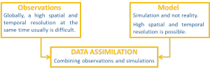 Figure 1: Principle of DA
(generated by Kerstin Schulze, University of Bonn)
Figure 2 illustrates how DA works in two steps. First, model states are simulated or predicted (by running the model code). Second, the prediction is compared to the observations. Depending on the assumed uncertainties of model prediction and observation, an updated optimal state estimate is calculated. It is also possible to combine the DA with the estimation (calibration) of model parameters in a combined Calibration and Data Assimilation (C/DA) framework.
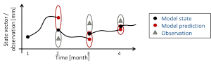
Figure 2: The two steps of DA
(generated by Kerstin Schulze, University of Bonn)
Within GlobalCDA, sequential DA methods will be implemented as often used for catchment-scale hydrological studies. However, we will, for the first time, develop a C/DA framework at global scale. Sequential methods predict model states to the actual observation epochs, and consider the data as soon as they are available, different from variational data assimilation. The result is used as the initial state for the next model prediction.
DA method – The Ensemble Kalman Filter (EnKF)
Within GlobalCDA, we will assimilate various data sets into the WaterGAP Global Hydrological Model (WGHM, see Project 2) using an Ensemble Kalman Filter (EnKF). The EnKF combines model prediction and observation in the Kalman gain matrix, which needs to account for the uncertainties as mentioned above. While the uncertainty of the observations can be derived from knowledge of the sensor and the measurement configuration, the uncertainty of the model prediction must be propagated using an ensemble method (Evensen 1994).
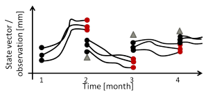 Figure 3: The EnKF
(generated by Kerstin Schulze, University of Bonn)
The ensemble members represent different realizations of the model simulation. The spread of the simulated values enables one to derive the model state uncertainty and takes the non-linearity of the model into account.